For ease of presentation, we first describe the personalized
communication algorithm for the case when the input is initially
evenly distributed amongst the processors, and return to the general
case in Section 3.3. Consider a set of n elements evenly
distributed amongst p processors in such a manner that no processor
holds more than  elements. Each element consists of a
pair
elements. Each element consists of a
pair  , where dest is the location to where
the data is to be routed. There are no assumptions made about the
pattern of data redistribution, except that no processor is the
destination of more than h elements. We assume for simplicity (and
without loss of generality) that h is an integral multiple of p.
, where dest is the location to where
the data is to be routed. There are no assumptions made about the
pattern of data redistribution, except that no processor is the
destination of more than h elements. We assume for simplicity (and
without loss of generality) that h is an integral multiple of p.
A straightforward solution to this problem might attempt to sort the elements by destination and then route those elements with a given destination directly to the correct processor. No matter how the messages are scheduled, there exist cases that give rise to large variations of message sizes, and hence will result in an inefficient use of the communication bandwidth. Moreover, such a scheme cannot take advantage of regular communication primitives proposed under the MPI standard. The standard does provide the MPI_Alltoallv primitive for the restricted case when the elements are already locally sorted by destination, and a vector of indices of the first element for each destination in each local array is provided by the user.
In our solution, we use two rounds of the transpose collective communication primitive. In the first round, each element is routed to an intermediate destination, and during the second round, it is routed to its final destination.
The pseudocode for our algorithm is as follows:
 , for
, for  ,
assigns its
,
assigns its  elements to one of p bins
according to the following rule: if element k is the first
occurrence of an element with destination j, then it is
placed into bin
elements to one of p bins
according to the following rule: if element k is the first
occurrence of an element with destination j, then it is
placed into bin  . Otherwise, if the last
element with destination j was placed in bin b, then
element k is placed into bin
. Otherwise, if the last
element with destination j was placed in bin b, then
element k is placed into bin  .
.
 routes the contents of bin
j to processor
routes the contents of bin
j to processor  , for
, for  . Since we
will establish later that no bin can have more than
. Since we
will establish later that no bin can have more than
 elements, this is the equivalent
to performing a transpose communication primitive with
block size
elements, this is the equivalent
to performing a transpose communication primitive with
block size  .
.
 rearranges the elements
received in Step (2) into bins according to each
element's final destination.
rearranges the elements
received in Step (2) into bins according to each
element's final destination.
 routes the contents of
bin j to processor
routes the contents of
bin j to processor  , for
, for  . Since
we will establish later that no bin can have more than
. Since
we will establish later that no bin can have more than
 elements, this is equivalent to
performing a transpose primitive with block size
elements, this is equivalent to
performing a transpose primitive with block size
 .
.
 by destination and then assigning
all those elements with a common destination j one by one to
successive bins
by destination and then assigning
all those elements with a common destination j one by one to
successive bins . Thus, the
  element
with destination j goes to bin
element
with destination j goes to bin  . Let
. Let  be the
number of elements a processor initially has with destination j.
Notice that with this placement scheme, each bin will have at least
be the
number of elements a processor initially has with destination j.
Notice that with this placement scheme, each bin will have at least
 elements with destination j,
corresponding to the number of complete passes made around the bins,
with
elements with destination j,
corresponding to the number of complete passes made around the bins,
with  consecutive bins having one additional
element for j. Moreover, this run of additional elements will begin
from that bin to which we originally started placing those elements
with destination j. This means that if bin l holds an additional
element with destination j, the preceding
consecutive bins having one additional
element for j. Moreover, this run of additional elements will begin
from that bin to which we originally started placing those elements
with destination j. This means that if bin l holds an additional
element with destination j, the preceding  bins will also hold an additional element with destination j.
Further, note that if bin l holds exactly q such additional
elements, each such element from this set will have a unique
destination. Since for each destination, the run of additional
elements originates from a unique bin, for each distinct additional
element in bin l, a unique number of consecutive bins preceding it
will also hold an additional element with destination j.
Consequently, if bin l holds exactly q additional elements, there
must be a minimum of
bins will also hold an additional element with destination j.
Further, note that if bin l holds exactly q such additional
elements, each such element from this set will have a unique
destination. Since for each destination, the run of additional
elements originates from a unique bin, for each distinct additional
element in bin l, a unique number of consecutive bins preceding it
will also hold an additional element with destination j.
Consequently, if bin l holds exactly q additional elements, there
must be a minimum of  additional elements in the bins preceding bin l for a minimum total
of
additional elements in the bins preceding bin l for a minimum total
of  additional elements distributed amongst the p
bins.
additional elements distributed amongst the p
bins.
Consider the largest bin which holds  of the
evenly placed elements and
of the
evenly placed elements and  of the additional elements, and
let its size be
of the additional elements, and
let its size be  . Recall that if a bin holds
 additional elements, then there must be at least
 additional elements somehow distributed
amongst the p bins. Thus,
additional elements somehow distributed
amongst the p bins. Thus,
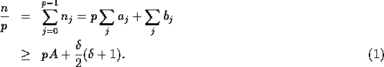
Rearranging, we get

Thus, we have that

Since the right hand side of this equation is maximized over  when
when  , it follows that

One can show that this bound is tight as there are cases for which the upper bound is achieved.
To bound the bin size in Step (4), recall that the number of
elements in bin j at processor i is simply the number of elements
which arrive at processor i in Step (2) which are bound for
destination j. Since the elements which arrive at processor i in
Step (2) are simply the contents of the  bins
formed at the end of Step (1) in processors 0 through p-1,
bounding Step (4) is simply the task of bounding the number of
elements marked for destination j which are put in any of the p
bins
formed at the end of Step (1) in processors 0 through p-1,
bounding Step (4) is simply the task of bounding the number of
elements marked for destination j which are put in any of the p
 bins in Step (1). For our purposes, then, we can
think of the concatenation of these p
bins in Step (1). For our purposes, then, we can
think of the concatenation of these p  bins as being
one superbin, and we can view Step (1) as a process in which
each processor deals its set of
bins as being
one superbin, and we can view Step (1) as a process in which
each processor deals its set of  elements bound for destination
j into p possible superbins, each beginning with a unique
superbin
elements bound for destination
j into p possible superbins, each beginning with a unique
superbin  . This is precisely the situation considered
in our analysis of the first phase, except now the total number of
elements to be distributed is at most h. By the previous argument,
the bin size for the second phase is bounded by
. This is precisely the situation considered
in our analysis of the first phase, except now the total number of
elements to be distributed is at most h. By the previous argument,
the bin size for the second phase is bounded by

 . The transpose primitive, whose analysis is
given in [7], takes
. The transpose primitive, whose analysis is
given in [7], takes  in the second step, and
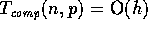
 in the last step. Thus, the overall complexity of our
algorithm is given by
in the last step. Thus, the overall complexity of our
algorithm is given by
for  . Clearly, the local computation bound is
asymptotically optimal. As for the communication bound,
. Clearly, the local computation bound is
asymptotically optimal. As for the communication bound,  is a lower bound as in the worst
case a processor sends
is a lower bound as in the worst
case a processor sends  elements and receives h
elements.
elements and receives h
elements.
