Experimental Results

For each experiment, the input is evenly distributed amongst the processors. The output consists of the elements in non-descending order arranged amongst the processors so that the elements at each processor are in sorted order and no element at processor is greater than any element at processor , for all i < j.

Two variations were allowed in our experiments. First, radix sort was used to sequentially sort integers, whereas merge sort was used to sort double precision floating point numbers (doubles). Second, different implementations of the communication primitives were allowed for each machine. Wherever possible, we tried to use the vendor supplied implementations. In fact, IBM does provide all of our communication primitives as part of its machine specific Collective Communication Library (CCL) [8] and MPI. As one might expect, they were faster than the high level SPLIT-C implementation.

  
Table i: Total execution time (in seconds) required to sort a variety of integer benchmarks on a 64-node Cray T3D.

  
Table ii: Total execution time (in seconds) required to sort a variety of integer benchmarks on a 64-node IBM SP-2-WN.

  
Table iii: Total execution time (in seconds) required to sort a variety of double benchmarks on a 64-node Cray T3D.

  
Table iv: Total execution time (in seconds) for required to sort a variety of double benchmarks on a 64-node IBM SP-2-WN.

Tables i, ii, iii, and iv display the performance of our sample sort as a function of input distribution for a variety of input sizes. In each case, the performance is essentially independent of the input distribution. These tables present results obtained on a 64 node Cray T3D and a 64 node IBM SP-2; results obtained from the TMC CM-5 validate this claim as well. Because of this independence, the remainder of this section will only discuss the performance of our sample sort on the single benchmark [U].

  
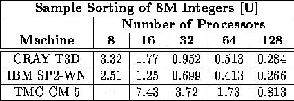
Table v: Total execution time (in seconds) required to sort 8M integers on a variety of machines and processors using the [U] benchmark. A hyphen indicates that particular platform was unavailable to us.

  
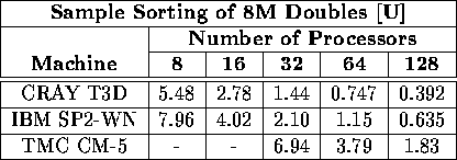
Table vi: Total execution time (in seconds) required to sort 8M doubles on a variety of machines and processors using the [U] benchmark. A hyphen indicates that particular platform was unavailable to us.

  
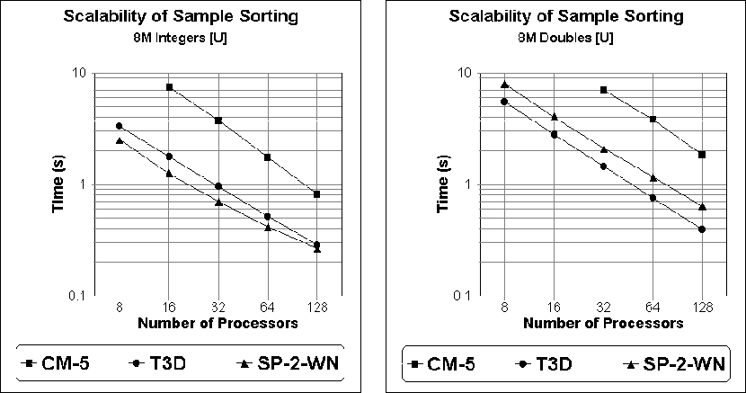
Figure 1: Scalability of sorting integers and doubles with respect to machine size.

The results in Tables v and vi together with their graphs in Figure 1 examine the scalability of our sample sort as a function of machine size. Results are shown for the T3D, the SP-2-WN, and the CM-5. Bearing in mind that these graphs are log-log plots, they show that for a fixed input size n the execution time scales almost inversely with the number of processors p. While this is certainly the expectation of our analytical model for doubles, it might at first appear to exceed our prediction of an computational complexity for integers. However, the appearance of an inverse relationship is still quite reasonable when we note that, for values of p between 8 and 128, varies by only a factor of . Moreover, this complexity is entirely due to the merging in Step (8), and in practice, Step (8) never accounts for more than of the observed execution time. Note that the complexity of Step 8 could be reduced to for integers using radix sort, but the resulting execution time would, in most cases, be slower.

The graphs in Figure 2 examine the scalability of our sample sort as a function of problem size, for differing numbers of processors. They show that for a fixed number of processors there is an almost linear dependence between the execution time and the total number of elements n. While this is certainly the expectation of our analytic model for integers, it might at first appear to exceed our prediction of a computational complexity for floating point values. However, this appearance of a linear relationship is still quite reasonable when we consider that for the range of values shown differs by only a factor of 1.2.

  
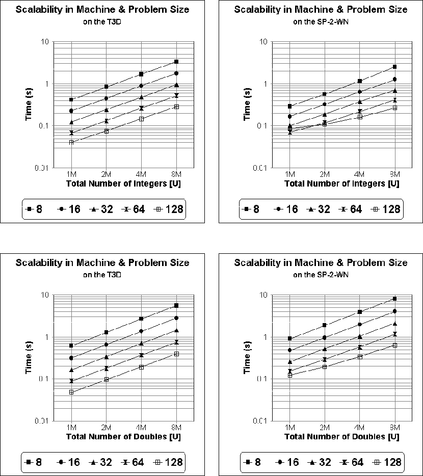
Figure 2: Scalability of sorting integers and doubles with respect to the problem size, for differing numbers of processors.

Next, the graphs in Figure 3 examine the relative costs of the eight steps in our sample sort. Results are shown for both a 64 node T3D and a 64 node SP-2-WN, using both the integer and the double versions of the [U] benchmark. Notice that for n = 64M integers, the sequential sorting and merging performed in Steps (3) and (8) consume approximately of the execution time on the T3D and approximately of the execution time on the SP-2. By contrast, the two transpose operations in Steps (2) and (7) together consume only about of the execution time on the T3D and about of the execution time on the SP-2. The difference in the distribution between these two platforms is likely due in part to the fact that an integer is 64 bits on the T3D while only 32 bits on the SP-2. By contrast, doubles are 64 bits on both platforms. For n = 64M doubles, the sequential sorting and merging performed in Steps (3) and (8) consume approximately of the execution time on both platforms, whereas the two transpose operations in Steps (2) and (7) together consume only about of the execution time. Together, these results show that our algorithm is extremely efficient in its communication performance.

  
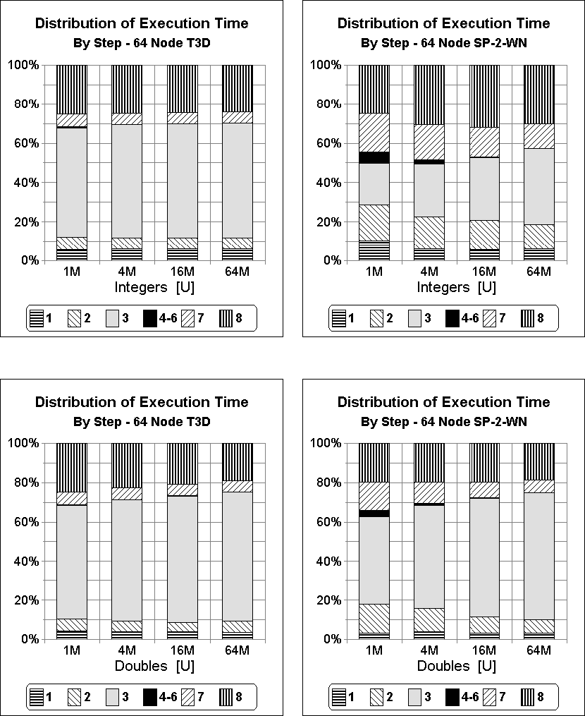
Figure 3: Distribution of execution time amongst the eight steps of sample sort. Times are obtained for both a 64 node T3D and a 64 node SP-2-WN using both the integer and the double versions of the [U] benchmark.

Finally, Tables vii and viii show the experimentally derived expected value (E) and sample standard deviation (STD) of the coefficients , , , and used to describe the complexity of our algorithm in Section 3. The values in Table vii were obtained by analyzing data collected while sorting each of the duplicate benchmarks [DD] and [RD] 50 times on a 64-node Cray T3D. For each trial, the values recorded were the largest occurrence of each coefficient at any of the 64 processors. By contrast, the values in Table viii were obtained by analyzing data collected while sorting each of the unique benchmarks [G], [B], [2-G], [4-G], and [S] 20 times. In every trial, a different seed was used for the random number generator, both to generate the benchmark where appropriate and to distribute the keys into bins as part of Step (1). The experimentally derived expected values in Table vii for , , , and agree strongly with the theoretically derived bounds for duplicate keys of , , , and for . Similarly, the experimentally derived expected values in Table viii for , , , and agree strongly with the theoretically derived bounds for unique keys of , , , and for . Note that expected values for and are actually less for duplicate values than for unique values, which is the opposite of what we might expect from the computed bounds. This might simply reflect our limited choice of benchmarks, or it may suggest that the bounds computed for duplicate are looser than those computed for unique values.

  
Table vii: Statistical evaluation of the experimentally observed values of the algorithm coefficients on a 64 node T3D using the duplicate benchmarks.

  
Table viii: Statistical evaluation of the experimentally observed values of the algorithm coefficients on a 64 node T3D using the unique benchmarks.